No audio available for this content.
A jammer-hunting UAV employs a radio frequency (RF) detection system and a navigation control scheme. The RF detection component uses a directional antenna and the unmanned aerial vehicle’s (UAV’s) ability to rotate to determine a bearing to the jammer. The navigation control scheme selects a trajectory for making bearing measurements that enable rapid jammer localization, based on three bearing calculation methods: max, cross-correlation, and a modification of max leveraging the shape of the antenna’s main lobe, known as max3.
By Adrien Perkins, Louis Dressel, Sherman Lo and Per Enge
Whether malicious or unintentional, GPS jamming events have already proven to disrupt airports and pose an increased risk to commercial aviation in the future. An important mitigation for this risk is the ability to rapidly locate and interdict the GPS jamming device.

antenna
mounted on underside of UAV.
The system must be capable of reliably determining jamming direction and quickly localizing the source in the semi-urban environments typically found in and around airports. This article examines both aspects.
In developing a localization algorithm, the measurements being made by the system can greatly impact performance. Using a directional antenna as the primary sensor, our multirotor platform Jammer Acquisition with GPS Exploration & Reconnaissance (JAGER) can measure the bearing to the jammer, which is the main input into the localization algorithm. Here we examine three different bearing calculation techniques from a gain pattern: max, cross-correlation and max3.
The closed-loop navigation controller uses the gathered information to determine where to go next to most quickly localize the jammer. In this article, the localization objective is modeled as a partially observable Markov decision process (POMDP) to determine the optimal route. The viability of this technique for locating the jammer source is demonstrated through flight testing in a simulated environment.
PROBLEM OVERVIEW
Because our vehicle is an agile, multirotor UAV, it can translate, climb, rotate and make received signal strength indicator (RSSI) measurements at the same time. It is computationally difficult to reason over such a large input space. Therefore, to simplify the problem, we constrain the vehicle to a constant altitude and assume a single, stationary jammer. We also decouple the problem into two actions: rotating — to measure bearing, and moving — to another measurement location.
This article focuses on the first action: How accurately can bearing be estimated if the vehicle samples RSSI values while rotating in place, and how can those measurements affect the decisions of where to rotate next?
POMDP Formulation. The problem of choosing successive rotation locations has been formulated as a POMDP. POMDPs are a principled approach to decision making and closed-loop control in stochastic domains.
At each time step, the problem can be described by a state s ϵ S, where S is the state space, or set of all possible states. To limit the size of the state space, the search area is split into a grid. A state consists of four state variables: the vehicle x-index xv, the vehicle y-index yv , the jammer’s x-index xj , and the jammer’s y-index yj. At each time step, the state is only partially observable — the jammer’s position is unknown.
At each time step, the vehicle can take some action a ϵ A, the set of available actions. In our formulation, the vehicle can travel to any of the neighboring grid cells, rotate in place to make a bearing measurement, or simply hover, resulting in 10 possible actions. After taking action a from state s, the problem will transition to some state s’.
At any time step, the state is unknown to the vehicle. Instead, it makes an observation o ϵ O, where O is the set of all possible observations. In our problem, these observations are the bearing measurements made when the vehicle rotates. To reduce the number of possible observations and computational complexity, the bearing measurements are discretized and include a “null” observation when the vehicle cannot determine a bearing.
The POMDP formulation includes an observation model Z(a, s’, o) = P(o | a, s’) describing the probability of making observation o after taking action a and transitioning to state s’. This probability is a function of the bearing measurement quality. Prior to the work presented here, it was assumed bearing measurements had zero-mean Gaussian noise with a 10-degree standard deviation. It was also assumed that if the vehicle rotated in the same grid cell as the jammer, it would receive the null measurement, because the space directly under the vehicle is outside the main lobe of its directional antenna. An updated observation model, using the characterization performed in this work, can be found in the section entitled “Effect on Algorithm.”
Although the vehicle is unaware of the true state, it maintains a probability distribution over the state space, called a belief, denoted b. After taking an action and making a new observation, Bayes’ law is used to update the belief. This updated belief is used in conjunction with policy π to determine the next action to take. A policy π(b) maps beliefs to actions.
Due to the large belief space, this research uses SARSOP, which allows a policy to be computed offline and uploaded to the vehicle before a mission. The vehicle then relies on this policy to make decisions while in flight.
Generating a policy requires a reward model that encourages the vehicle to perform certain actions. In our formulation, we reward the vehicle when it stops in the grid cell containing the jammer. This encourages the vehicle to first find the jammer, which is our goal. We give penalties for movement and rotations to reflect the time taken to perform them.
EXPERIMENTAL SETUP
Our jammer-hunting UAV, JAGER, is a commercially available DJI S1000. The S1000 is made to carry film-grade cameras, but we’ve modified it to carry our experimental payload. For control and navigation, the vehicle is equipped with a Pixhawk autopilot system running a custom version of the PX4 firmware. The Pixhawk has sensors to determine the vehicle’s attitude, altitude, and position. The localization decisions are made on the flight computer, which is an Odroid-U3 ARM-based computer that communicates with the autopilot throughout the flight. All signal strength measurements are made with a directional yagi antenna connected to the RN-XV WiFly module. A schematic of this configuration and the flow of information can be seen in Figure 1.

Given the small size of this payload, the flight time achieved during testing was 20 minutes on 4 pounds of batteries (two 6-cell 8000-mAh batteries).
Signal Source. Due to restrictions on active interference with GPS signals, a 2.4-GHz Wi-Fi router was used as a proxy jammer for all our flight testing. The Wi-Fi router was placed on the ground at a surveyed location. In these tests, GPS was used for navigation as we are still developing alternate and GPS jamming resistant navigation.
Antenna. A single the L-com HG2409Y yagi antenna was used for this experiment. This 2.4-GHz Wi-Fi antenna has a 60-degree beam width both horizontally and directionally as shown in Figure 2. As depicted in the opening graphic, the antenna was mounted below the vehicle in order to have the clearest view to a ground based signal. Furthermore, the antenna is placed angled down at 30 degrees in order to have the main lobe of the antenna extend out to the horizon. This also leaves a cone underneath the vehicle with a weak signal that was aimed to be leveraged as a null measurement when over the jammer.

While we are currently using a Wi-Fi-based system to stand in for GPS, we eventually plan to test this system on a true GPS jammer. Despite the different frequencies, the same methodology and approach will be able to be used when localizing a GPS jammer. The biggest change the system will require is the antenna required to make bearing measurements. For Wi-Fi, we have been able to successfully use an off-the-shelf directional antenna, but for GPS either a custom directional antenna or a dual-antenna solution will be needed.
Measurements. Throughout the UAV’s flight, the directional antenna makes RSSI measurements at 2 Hz. To calculate bearing from a given location, the vehicle simply rotates at a rate of 15 degrees/second at that position and combines all of the RSSI measurements using magnetometer data to form the antenna’s gain pattern. This gain pattern can then be used to estimate the bearing of the signal source from that given position. In this paper that bearing calculation is done with three different methods: max, cross-correlation and max3.
The max method simply finds the maximum RSSI value in the measured pattern and uses that heading as the bearing to the jammer.
The cross-correlation method normalizes the measured pattern and compares it with the known truth pattern for the antenna. The truth pattern is shifted by some angle γ. The cross-correlation is computed for every possible shift γ. The shift yielding the highest cross-correlation coefficient is taken to be the bearing to the jammer.
To get our truth pattern, we sampled RSSI every 10 degrees at distances ranging from 10 to 40 meters, normalized the resulting patterns, and took the mean of these normalized patterns.
The max3 method is an improvement on the max method where the bearing is the mean of the bearing of the two crossings of 3 dB below the maximum RSSI value for the pattern, as depicted in Figure 3.

Flight Area. Test flights were performed at the Joint Interagency Field Experimentation (JIFX) event hosted by the Naval Postgraduate School. Most measurement were taken at an altitude of 100 feet AGL with a handful of measurements made near the signal source at an altitude of 50 feet AGL. When the localization algorithm was tested, a 9 by 9 grid (each cell 11 meters on a side) was used as the world, with the signal source located in the top right cell and the vehicle starting in the center cell, 62 meters from the signal source.
RESULTS
During flight tests with the JAGER vehicle, 88 different experimental gain patterns were created, and bearing calculations were made with each of the three previously described methods.
The POMDP-based localization algorithm was successfully executed to locate the signal source. Leveraging the performance results of the cross-correlation and max3 methods, the model for the POMDP was updated and produced a significantly different flight profile. In addition to the POMDP-based localization algorithm, a baseline algorithm was also used to demonstrate the advantages of the POMDP-based algorithm.
Effects of Distance. Throughout the experiment, measurements were made at distances from the signal source ranging from directly overhead to almost 350 meters away. Figure 4 shows all the locations in which measurements were taken during flight tests, with the signal source in the center of the main grouping. Each marker represents one measurement, and its color represents roughly the maximum RSSI value measured at each location. As expected, as the vehicle traveled further from the signal source, the maximum RSSI value measured dropped. Near the signal source, the signal is no longer captured by the main lobe, which result in poor measurements, as can be seen by the grouping of orange and red markers near the source.

MEASUREMENT CLASSIFICATION
Because of effects of distance on the measurements and the configuration of the antenna on the vehicle, all measurements were split into three classifications: near, ideal and far.
Near. Near measurements are measurements made where the signal source is within the cone underneath the vehicle, where the main lobe of the antenna no longer reaches. When the signal source was near the vehicle, we did not obtain null measurements, but rather obtained gain patterns such as the one shown in Figure 5. These gain patterns do not resemble the ideal gain pattern of the antenna due to the noise in the measurements from the signal source not being picked up by the main lobe, making it challenging for any of the bearing calculation methods to successfully determine the bearing.

Far. Far measurements are any measurement further than 200 meters from the signal source. At these distances, the RSSI measurements were at or below the receiver sensitivity. At these distances, the resulting gain patterns no longer had enough measurements to clearly resemble the ideal gain pattern of the antenna. Figure 6 shows a gain pattern from 250 meters away with a true bearing of 267 degrees and demonstrates the partial pattern that is measured. The cross-correlation estimate of 182 degrees suffers from the inability to match the partial pattern with the required truth pattern. On the other hand, the simplicity of the max and max3 methods result in more accurate estimates of 271 and 285 degrees, respectively.

Ideal. This leaves the ideal category, which is any measurement made between near and far. At this distance, the signal source was able to both be within the main lobe of the antenna and within reasonable rage of the WiFly’s sensitivity. In the ideal range, the gain patterns produced resemble the true pattern of the antenna, as shown in Figure 7.

In the flight tests, the majority of the measurements taken were in the ideal range. Only a few measurements were made in the far range so no detailed analysis is presented for measurements in the far range.
BEARING METHODS PERFORMANCE
An overview of the standard deviation of all the results can be seen in TABLE 1.


The proper characterization of the antenna is vital to the performance of the POMDP localization algorithm. Using the results presented with the max3 and cross-correlation methods, the POMDP model can be updated to better reflect the measurements in order to improve the flight profile for localization.
Max. The max method is the simplest method used to calculate the bearing to the signal from a given set of measurements. This method is also the reason for the poor performance in calculating the bearing. This method can too easily pick a wrong estimate if there is a spike in what should be a smooth main lobe as depicted in Figure 11. These spikes cause a large spread in the errors in calculating bearing seen in Figure 8.

Cross-Correlation. Cross-correlation is the most complex of the methods used and in the ideal range is one of the best performing methods (on par with the max3 method).
The overall performance of the cross-correlation suffered from the poor performance near and far from the router. Since this method requires a known truth pattern, when the experimental measurements don’t yield enough results to create a full pattern, the cross-correlation can mistakenly identify the partial pattern for a side lobe instead of a main lobe as was seen in Figure 6.
In the ideal range, it greatly outperforms the max method as expected. When looking at the bearing error shown in Figure 9, it can be seen that the errors are much more tightly grouped near zero than those seen in Figure 8 for the max method. The outliers for the far measurement caused by a failure to match the partial patterns to the truth can also be clearly seen in this figure.

The increase in performance from near to ideal can clearly be seen in Table 1, where the standard deviation of the error is significantly smaller for the ideal case.
Max3. Max3 is the strongest of the three bearing calculation methods tested; overall, it performed the best and max3 has the advantage of simplicity over cross-correlation. It can perform on par with cross-correlation in the ideal range as can be seen by the similarly close error groupings in Figures 12 (max3) and 9 (cross-correlation) and by the similar standard deviations seen in Table 1.

The benefit over the cross-correlation method of not requiring a known truth pattern allows max3 to perform well when the number of measurements is very small and the gain pattern is mostly incomplete. However, max3 has difficulty making accurate bearing calculations when close to the router, though not as badly as the other two methods.
The advantage max3 has over the simple max is well illustrated in Figure 11. While the gain pattern looks very promising, there is a spike along the otherwise mostly smooth main lobe at 116 degrees. This spike is off from the true 92-degree bearing which results in the max method estimating an incorrect bearing. By taking the mean of the bearing of the two crossing points 3 dB below the max (marked in blue x’s), effects from spikes like the ones depicted are reduced allowing for a much better estimate of 93 degrees.

Through this characterization, the performance seen from max3 can be used to update the POMDP model to improve the localization algorithm, as described in section “Effect on Algorithm.”
ALGORITHM PERFORMANCE
One of the goals of our flight tests was to determine the feasibility of the POMDP approach and begin to understand the performance of the POMDP method. A simple baseline method was used for comparison. The baseline method used in this test was a variable step greedy algorithm that moved in the direction of the calculated bearing (using the max method) with a variable step size. The step size was based on the similarity between measurements, resulting in an increased step size when moving in the same direction toward the signal source.
Using this baseline method, JAGER was able to move toward the location of the signal source, and with the assistance of a user monitoring the behavior, was able to locate the signal source. The flight path of the vehicle for this test can be seen in Figure 13.
With a user in the loop with this baseline method, a good estimate of the location can be determined by watching the behavior of the vehicle. Looking at Figure 13, it can be seen that the vehicle kept crossing its path near one location, which can be determined to be an estimate of the location of the signal source. It is worth noting that the baseline method does take four steps to get in the region of the signal source, and then another four or five steps for the user to be confident that the vehicle is in the vicinity of the signal source.

POMDP Localization. With a baseline determined, the POMDP approach was executed from the same starting location and used the simple max bearing method for determining bearing from each location. This localization took a mere two steps and three measurements to be able to locate the signal source. Figure 14 shows the state updates as the vehicle made subsequent measurements. After the first measurement is made at the starting location, the vehicle is able to immediately narrow down the location of the signal source to a small region within the grid.

Unlike the simple method of moving slowly in the direction of the max bearing, the POMDP method can make large changes in order to get to the next best location to make a measurement.
When running this algorithm, we had an assumption that when the vehicle is in the same cell as the signal source, a null measurement would be made. Unfortunately, near and over the signal source resulted in noisy measurements, and that noise resulted in location of the signal source being off by one cell.
Effect on Algorithm. The experiments in this paper were performed to obtain a better observation model for the localization algorithm. Previously, the model assumed 10-degree noise except when the vehicle was in the same cell as the jammer; there the modeled assumed a null measurement would be obtained. These assumptions were used in the experimental trajectory shown in Figure 15 and affected the selected trajectory. The vehicle always moved toward regions with high probability of containing the jammer (the dark red cells). Because we assumed that rotation would only yield a null measurement when over the jammer, receiving a null observation after rotating would convince the vehicle that the jammer was in its current cell. For this reason, the vehicle moves to regions with high probability of containing the jammer; it hoped to receive this high-information measurement and solve the problem with a single rotation.

Experimental results have shown that measurement noise increases greatly close to the jammer. Our new model assumes 40-degree noise if the jammer is in any of the adjacent grid cells when the vehicle rotates, and 13-degree noise if the jammer is farther away. If the vehicle rotates in the same cell containing the jammer, it no longer receives a null measurement. Instead, it can receive any measurement with uniform probability.
Generating a policy with this new model leads to different trajectories. A simulated rerun of the experimental trajectory from Figure 15 is shown in Figure 16. The vehicle avoids the darker cells, which indicate higher probability of containing the jammer. Instead the vehicle chooses to rotate in cells it believes are farther away from the jammer to avoid possible measurement noise.

CONCLUSION
This article presents the development of the localization component of a UAV to locate the source of a GPS jamming signal. For the scenarios tested, modeling the localization as a POMDP is a viable solution that can locate a static signal source in very few steps. It is faster and has greater confidence than a simple, greedy search baseline solution.
Through extensive test flights using a single directional antenna and rotation-based measurements, three different bearing methods have been analyzed. All three methods suffered when near the signal source due to the antenna reception pattern, which resulted in very noisy measurements. Of the three, max3 and cross-correlation fared the best in the ideal distance from the signal source. Max3 was able to outperform cross-correlation when the UAV was far from the signal source due to the limitations of cross-correlation requiring a truth pattern for correlation. However, cross-correlation can also provide a useful correlation coefficient that can be used in the future to merge several bearing calculation methods.
The characterization of antenna bearing performance is a vital component to the localization process. The characterization affects the optimal behavior determined by POMDP. When we changed our initial assumptions about measurement performance near the jammer to one better informed by our tests, the actions determined POMDP resulted in a significantly different profile.
ACKNOWLEDGMENTS
The authors gratefully acknowledge the Naval Postgraduate School for providing an unmatched space to be able to perform test flights of the JAGER system at the Joint Interagency Field Experimentation events. The authors would also like to thank the Stanford Center for Position Navigation and Time (SCPNT) and its members for supporting this work.
MANUFACTURERS
The JAGER UAV airframe is a S1000 octocopter by DJI Innovations; the flight batteries are a 8000 mAh model by Hextronik; the autopilot hardware and GPS antenna is a Pixhawk by 3D Robotics, Inc.; the autopilot software is based on PX4 by Pixhawk.org. The tracking hardware comprises a 2.4 GHz Yagi antenna from L-com; an RN-XV Wi-Fi module by Roving Networks; and an Odroid-U3 computer by Hardkernel Co.
Adrien Perkins is a Ph.D. candidate in the GPS Research Laboratory at Stanford University, where he received his MSc. in aeronautics and astronautics.
Louis Dressel is a Ph.D. candidate in the Aeronautics and Astronautics Department at Stanford, where he works on a joint project with the Stanford Intelligent Systems Lab and the GPS Research Laboratory.
Sherman Lo is a senior research engineer at the Stanford University GPS Laboratory.
Per Enge is a professor of aeronautics and astronautics at Stanford, where he directs the GPS Research Laboratory.
This article is based on a technical paper presented at the 2015 ION-GNSS+ conference in Tampa, Florida.