Listen to this content
Ionospheric delay remains a significant error source in GNSS positioning, particularly for single-frequency users and during periods of enhanced space weather activity (Dabbakuti, 2021). While global and regional ionospheric models provide large-scale corrections, they often fail to represent localized ionospheric variability at individual receiver locations (Jee et al., 2010; Osanyin et al, 2025).
Consequently, residual ionospheric errors persist in positioning solutions, degrading accuracy for applications including precise point positioning (PPP), real-time navigation, and single-frequency GPS users (Biswas et al., 2022). Hence, accurate modeling of the ionosphere is essential in tackling the principal challenges in high-precision GNSS positioning.
Vertical total electron content (VTEC), a key driver of ionospheric delay, exhibits strong nonlinear temporal variability controlled by solar radiation, geomagnetic activity, seasonal effects, and local electrodynamics (Osanyin et al., 2023; Seemala et al., 2023). Capturing this variability at individual GNSS stations poses a significant challenge. Advances in artificial intelligence (AI), i.e., machine learning (ML) techniques have emerged over the decades as powerful tools for approximating complex non-linear systems and deterministic geophysical processes, while significantly reducing computational cost (Sarker, 2021). As such, they have successfully replaced repeated full-scale numerical simulations by learning input-output relationships directly from data (Zhang et al., 2025). This paradigm shift is particularly relevant for ionospheric modeling, where long-term GNSS observations provide rich time series well suited for data-driven learning.
Time series forecasting traditionally relies on statistical models such as autoregressive (AR), moving average (MA), autoregressive moving average (ARMA), and autoregressive integrated moving average (ARIMA), which model future values as linear functions of past observations (Kaselimi et al., 2020). They have been widely employed to predict VTEC by extrapolating historical observations. Nonetheless, the classical approaches are inherently limited by assumptions of linearity, stationarity and short-term memory, which restrict their ability to capture complex ionospheric dynamics, particularly during disturbed conditions and over longer prediction horizons. To address these limitations, this study adopts a deep learning-based framework using long short-term memory (LSTM) neural networks for station -pecific VTEC prediction. Unlike conventional statistical models, LSTM networks are specifically designed to learn non-linear temporal relationships and retain long-term memory in sequential data (Hochreiter and Schmidhuber, 1997).
Essentials
LSTM neural networks for prediction have emerged as a powerful tool for time-series prediction (Hochreiter and Schmidhuber, 1997). LSTM is a type of recurrent neural networks (RNNs) that takes sequences of information and uses recurrent mechanisms and gate techniques (see Figure 1). RNNs are well known for their ability to process single data points and entire data sequences (Gonzalez and Yu, 2018). The LSTM model has various forms for different types of data inputs. The basic condition of LSTM modeling is that all inputs and outputs are independent of each other. The key to the LSTMs is the cell state, which is protected and controlled by the forget, input and output gates, respectively (Gonzalez and Yu, 2018).
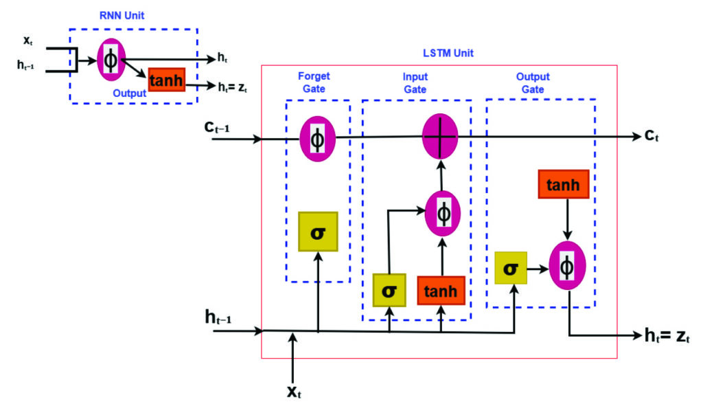
FIGURE 1 Comparison of recurrent neural network (RNN) and long short-term memory (LSTM) structures.
Training deep learning models remains computationally demanding despite their fast prediction capability. LSTM networks consist of interconnected layers with numerous trainable parameters that must be optimized iteratively to accurately capture temporal dependencies in the data. Training typically involves large historical datasets spanning multiple years, which is necessary to expose the model to varying ionospheric conditions, but also increases computational effort (Thompson et al., 2020). The optimization process relies on iterative algorithms such as stochastic gradient descent and variants, requiring repeated forward and backward passes through the network. As the depth of the model and the length of input sequences increase, so does the demand for memory and processing power. These challenges are particularly relevant when training is performed using graphics processing units (GPUs), where memory limitations and data transfer overhead must be carefully managed (Sarker, 2021).
Like all neural networks, LSTM has trainable parameters (weights and biases). These parameters are optimized by minimizing a loss function using gradient-based optimization. Due to its ability to learn time sequences, gradients must be propagated across time steps, not only across layers. This process is accomplished using backpropagation through time, which computes gradients of the loss with respect to all parameters and accumulates gradients across the sequence. The major advantage of LSTM is the use of its gating mechanism in mitigating vanishing gradients, making backpropagation practical for long time series such as VTEC (Adekunle et al., 2025; Hochreiter and Schmidhuber, 1997; Noor and Ige, 2025).
In recent years, LSTM networks have achieved impressive results in modeling complex physical systems characterized by strong non-linearity and long-term temporal dependencies. Notably, LSTM-based approaches have been successfully applied to atmospheric and geophysical time series, demonstrating superiority in predictive skill compared to traditional empirical and statistical models (see Reddybattula et al. (2022 and references therein). These research results show the capability of LSTM to capture diurnal, seasonal, and storm-time variations. By leveraging historical GNSS-derived VTEC time series, LSTM-based models can adaptively capture both regular ionospheric patterns and transient disturbances, enabling more accurate and robust VTEC forecasts. This data-driven approach directly supports improved ionospheric correction in GNSS positioning, offering a practical and scalable solution to overcome the shortcomings of traditional time series methods.
This study focuses a station-specific vertical total electron content (VTEC) prediction framework based on long short-term time series. The proposed framework treats VTEC prediction as a supervised regression problem. A sequence of past VTEC observations is used to predict future values over one or multiple forecast horizons. Also, emphasis is placed on methodology clarity, practical implementation, and positioning relevance.
Elements: TEC estimation from GNSS measurements
For the purpose of forecasting local VTEC using time series analysis, this study utilized the GPS dataset provided by the Brazilian Institute for Geography and Statistics (RBGE; www.ibge.gov.br/en/) over Santa Maria (SMAR; -20.72o, 306.28o), a station located in Brazil over the period of 10 years from January 2010 to December 2019.
VTEC data were derived from dual-frequency GPS observations at the selected station using the standard ionospheric processing techniques, including slant TEC estimation, instrumental bias correction, and mapping to vertical TEC. For more details, readers can consult the GPS-TEC analysis software developed by Seemala and Valladares (2011), which has been employed in this study for TEC processing. The time resolution is selected to be 15 minutes following an average over a sampling interval of 30 seconds. The resulting VTEC time series provides a continuous record of ionospheric variability with a fixed temporal resolution.
Station-specific LSTM modeling framework
A structured deep learning workflow for station-specific VTEC prediction has been adopted using the LSTM framework. The overall methodology follows a sequential pipeline consisting of data collection, preprocessing, feature engineering, model training, evaluation, validation, and deployment. This workflow ensures reproducibility, minimizes information leakage, and facilitates integration into GPS positioning engines. The focus is on time series learning at a single station, where temporal dependencies dominate and spatial smoothing from regional or global models is undesirable.
Data preparation and model training
High-quality input data are essential for stable LSTM training. The extracted VTEC time series are preprocessed to remove cycle slips, mitigate differential code biases, and ensure consistent temporal sampling. As shown in Figure 2, for this model (as variations can be considered), the dataset has been divided into training (80%), validation (10%), and testing (10%). The validation is mostly required during training the LSTM deep learning model to ensure generalization and prevent overfitting. Furthermore, preprocessing aims at ensuring capability of the model in handling missing data and temporal consistency checks.
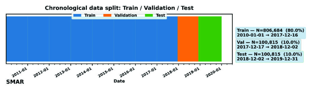
FIGURE 2 Chronological splitting of VTEC dataset for machine learning.
Feature engineering mainly converts raw VTEC observations into structured model inputs such as local time (LT) and day-of-year (DOY) features. These features are normalized prior to training, although normalization is applicable to only the training dataset to avoid future leakage. The model consists of an input layer whose dimension equals the number of input features, followed by a single LSTM layer with 64 memory cells to learn temporal dependencies in the input sequence. A dropout layer with a rate of 0.2 is applied to mitigate overfitting during training. The LSTM representation is then passed to a fully connected (Dense) regression head with nout neurons, where nout equals the number of forecast lead times. Model training minimizes the Huber loss function using gradient-based optimization, while performance is evaluated using RMSE. The optimizer updates the network weights iteratively to reduce the forecast error across the training samples. Early stopping and regularization are applied to further prevent overfitting, particularly during periods of low ionospheric variability. The final outputs are the predicted VTEC at multiple lead times (in this experiment: 30, 60, 120 and 180 minutes). The trained model is suitable for deployment in near real-time ionospheric correction systems: once operational, it ingests the most recent VTEC observations and produces short-term forecasts that can be integrated into GNSS positioning workflows, particularly for single-frequency applications and PPP.
Performance evaluation and baseline comparison
For practical assessment, the LSTM-based predictions are evaluated against commonly used baseline models, including persistence (using the trained model with new data) and skill (the ability of the model to make predictions). These baselines represent the minimum performance expected in operational GNSS ionospheric modeling and serves as internal validation of the overall model’s performance. Evaluation metrics include, but are not limited to, root mean square error (RMSE), mean absolute error (MAE), and relative improvement over persistence (skill). Figure 3 compares the predictive performance of the proposed LSTM model against the persistence baseline on the independent dataset. RMSE increases over time, while persistence largely deviates from the LSTM model, showing the great strength and capability of the LSTM model for time series prediction over the Santa Maria station. For instance, the RMSE of the LSTM model increases from 0.24 TECU to 1.15 TECU from 30 minutes to 3 hours lead time, while that of persistence ranges from 0.41 TECU to 2.25 TECU, respectively.
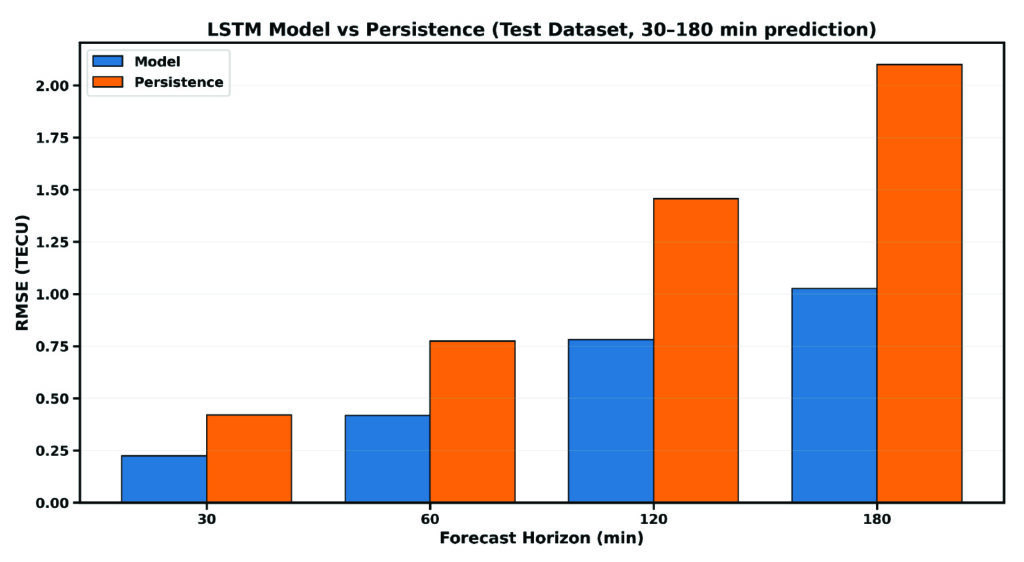
FIGURE 3 Comparison between the RMSE of the LSTM model and persistence for single-station VTEC prediction.
For further evaluation, day-to-day variation of VTEC at 60 minutes lead time is shown in FIGURE 4. GPS TEC (orange curves) shows a strong diurnal cycle with expected daily peaks, while forecast (blue curves) matches these peaks across months, indicating that the LSTM captures the key deterministic component of TEC variability. TABLE 1 or the embedded metrics in Figure 4 summarizes an overall accuracy of the LSTM model using the performance metrics: MAE, RMSE, Bias, R, and skill. MAE and RMSE values change with season — with the lowest reported in July.
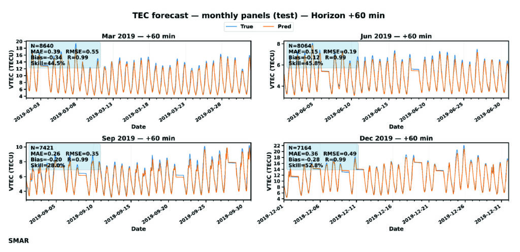
FIGURE 4 Day-to-day variation of VTEC at 60 minutes forecast during July to December 2019. The embedded metrics show the performance of the LSTM model for each month of the testing dataset.
Error increases toward December with the largest RMSE in March (0.549 TECU). September shows moderate error levels. Also, correlation is consistent across all months, which confirms the model’s capability to capture TEC changes and day-to-day variability patterns. The model is nearly unbiased as the bias is consistently close to zero, meaning that the LSTM does not drift systematically and shows that the model underpredicts GPS VTEC. This characteristic is important for operational GNSS corrections, because biased VTEC forecasts would translate to persistence positioning errors. Going by the skill values, even at 60 minutes forecast, the model provides ~27%-52% improvement over persistence. This result implies a major indicator of real predictive ability, especially for GNSS applications.
Statistical validation
Figure 5 presents the diagnostic of the validation dataset for the SMAR station at a 60-minute forecast horizon. It combines the distribution of prediction residuals (left) and density-based scatter comparison between predicted and observed VTEC values. These analyses help explain the overall agreement of the LSTM model forecast during validation.
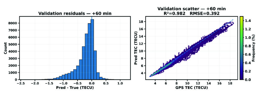
FIGURE 5 Validation diagnostics at 60 minutes forecast horizon. (Left) Histogram of prediction residuals. (Right) Density scatter of predicted versus observed TEC.
The residual distribution is mostly concentrated near zero, which implies that most predictions deviate only slightly from observations. The right plot shows the scatter density plot of predicted VTEC against observed GPS VTEC. The points are tightly clustered along the dashed line, indicating that the model corresponds very well (98.2%) to the TEC variance in the validation period. Also, a RMSE of 0.39 TECU reflects a relatively low magnitude error. These findings support the reliability of the proposed LSTM model for VTEC forecasting.
Implications for GNSS Positioning
The cumulative distribution function (CDF) of the absolute equivalent L1 error, denoted by |∆ρ|, for the Santa Maria station at a forecast horizon of 60 minutes is shown in Figure 6.
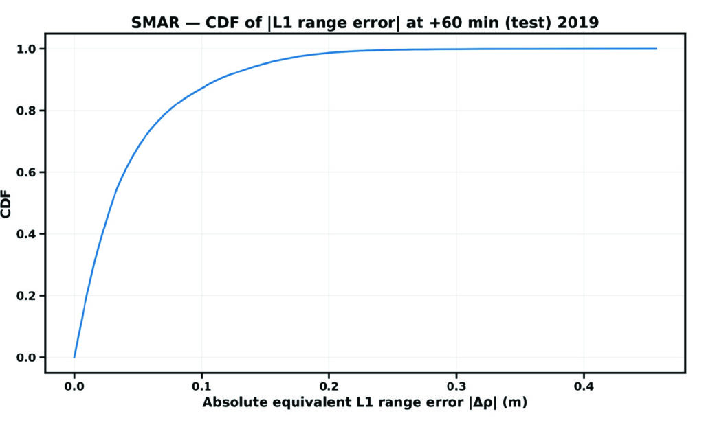
FIGURE 6 CDF of residual VTEC equivalent L1 ranging error at the single station.
The CDF provides a direct positioning-relevant interpretation of model performance. The steep rise at small error values indicates that most samples exhibit low residual range errors, demonstrating strong correlation performance.
Evolutionary
This study demonstrates that LSTM-based machine learning provides a practical and effective approach for station-specific GNSS VTEC prediction during low solar activity. The LSTM model accurately reproduces diurnal and seasonal VTEC variability at the station level. Forecast skill remains stable across increasing horizons, while significant RMSE reductions over persistence confirm the model’s predictive value, supporting the feasibility of LSTM-based station-specific VTEC forecasting for operational GNSS applications. By leveraging historical GPS-derived VTEC time series, LSTM neural networks capture complex temporal dependencies that are difficult to model using conventional techniques. This approach offers a valuable complement to existing ionospheric correction models and represents a promising direction for future GNSS positioning systems. The results presented in Table 1 confirm that the proposed LSTM algorithm can derive an accurate predictive model as far as a 3-hour forecast. The proposed approach improves long-term ionospheric prediction and enhances positioning accuracy.
| Month | MAE (TECU) | RMSE (TECU) | Bias (TECU) | R | Skill |
| Mar | 0.39 | 0.55 | -0.34 | 0.993 | 44.5 |
| June | 0.15 | 0.18 | -0.12 | 0.994 | 25.8 |
| Sep | 0.26 | 0.35 | -0.20 | 0.986 | 28.0 |
| Dec | 0.36 | 0.49 | -0.28 | 0.994 | 52.8 |
Table 1 Comparison of VTEC performance metrics of the LSTM model at 60 minutes forecast.
While the results demonstrate the potential of AI-based modeling for station-specific VTEC prediction, further investigation is required to assess its limitations. Future research will investigate the sensitivity and robustness of the data-driven approach under extreme geomagnetic storm conditions and maximum solar activity considering multiple stations over the same region. These experiments will help evaluate the LSTM-based modeling reliance for a better positioning GPS accuracy. In addition, combining efficient training strategies with LSTM-based temporal learning offers a practical and scalable solution to station-specific VTEC prediction. The resulting models will bridge the gap between computationally expensive physics-based approaches and overly simplified empirical models, providing accurate, localized ionospheric corrections that directly enhance GPS positioning performance. Therefore, the Bayesian optimization technique would be integrated during model’s training to tune LSTM hyperparameters (Adekunle et al., 2025), with the aim of reducing computational cost and improving convergence and generalization in station-specific ionospheric modeling. It is very likely that machine learning will play a significant role in near-term ionospheric modeling/prediction for GNSS.
Dr. Taiwo Osanyin is a Ph.D. visitor at York University, Toronto, Canada. Her research interests include space physics, atmospheric sciences, statistics, and modeling of the upper atmosphere. Osanyin received a Ph.D. in space geophysics from the National Institute for Space Research, Brazil, an M.Sc. in nuclear science and engineering from Obafemi Awolow University, Nigeria, and a B.Sc. in engineering physics from Obafemi Awolow University, Nigeria.
Sunil Bisnath is a full professor in the Department of Earth and Space Science and Engineering at York University in Toronto. For more than 25 years, he has been actively researching precise GNSS-focused positioning and navigation solutions and applications. He holds an Honors Bachelor of Science degree and master of science degree in surveying science from the University of Toronto and a Ph.D. in geodesy and geomtics engineering from the University of New Brunswick.
• Adekunle AA, Fofana I, Picher P, Rodriguez-Celis EM, Arroyo-Fernandez OH, Zemouri R. (2025). Optimizing deep learning predictive models: A comprehensive review of RNN and its variant architectures. Applied Soft Computing. Oct 9:114015.
• Biswas T, Banerjee P and Paul A (2022). Impact of low-latitude ionospheric effects on precise position determination. Radio Science, 57(4): 1-11.
• Dabbakuti JK (2021). Modeling and optimization of ionospheric model coefficients based on adjusted spherical harmonics function. Acta Astronautica, 182: 286-294.
• Gonzalez J and Yu W (2018). Non-linear system modeling using LSTM neural networks. IFAC-PapersOnLine, 51(13): 485-489.
• Hochreiter S and Schmidhuber J (1997). Long short-term memory. Neural Computation, 9:1735-1780.
• Jee G, Lee HB, Kim YH, Chung JK, Cho J (2010). Assessment of GPS global ionosphere maps (GIM) by comparison between CODE GIM and TOPEX/Jason TEC data: Ionospheric perspective. Journal of Geophysical Research: Space Physics. 115: A10.
• Kaselimi M, Voulodimos A, Doulamis N, Doulamis A, Delikaraoglou D. (2020). A causal long short-term memory sequence to sequence model for TEC prediction using GNSS observations. Remote Sensing. 12(9): 1354.
• Noor MH and Ige AO (2025). A survey on state-of-the-art deep learning applications and challenges. Engineering Applications of Artificial Intelligence. 159: 111225.
• Osanyin TO, Candido CM, Becker-Guedes F, Migoya-Orue Y, Habarulema JB, Obafaye AA, Chingarandi FS, Moraes-Santos SP (2023). Performance of a locally adapted NeQuick-2 model during high solar activity over the Brazilian equatorial and low-latitude region. Advances in Space Research. 72(12): 5520-38.
• Osanyin TO, Maria Nicoli Candido C, Becker-Guedes F, Migoya-Orue Y, Habarulema JB (2025). Ingestion of GNSS-Derived-TEC Into NeQuick 2 Model Over South America. Space Weather. 23(12): e2024SW004212.
• Reddybattula KD, Nelapudi LS, Moses M, Devanaboyina VR, Ali MA, Jamjareegulgarn P, Panda SK (2022). Ionospheric TEC forecasting over an Indian low latitude location using long short-term memory (LSTM) deep learning network. Universe. 8(11): 562.
• Sarker IH (2021). Deep learning: a comprehensive overview on techniques, taxonomy, applications and research directions. SN Computer Science. 2(6): 1-20.
• Seemala GK, Katual I, Kapil C, Vichare G (2023). Seasonal and solar activity dependence of TEC over Bharati station, Antarctica. Polar Science. 38: 101001.
• Seemala GK, Valladares CE. Statistics of total electron content depletions observed over the South American continent for the year 2008 (2011). Radio Science. 46(05): 1-4.
• Thompson Neil C, Kristjan G, Keeheon L, Manso Gabriel F (202). The computational limits of deep learning. Cornell University, arXiv:2007.05558, 10: 2.
• Zhang R, Li H, Shen Y, Yang J, Li W, Zhao D, Hu A (2025). Deep learning applications in ionospheric modeling: progress, challenges, and opportunities. Remote Sensing. 17(1): 124.