Dead Reckoning Keeps GPS in Line: Vehicle Positioning in Urban Environments


 |
Inaccurate positions from GPS receivers limit their usefulness in many urban environments. The causes for this inaccuracy include:
- multipath: reflections of GPS signals from buildings
- shadowing: poor signal propagation in cities (urban canyons) or under dense vegetation
- signal loss in tunnels, undercover car parks, and covered roadways
- extended time to first fix (TTFF) in poor signal areas
- dynamic limitations, such as maximum jerk (rate of change of acceleration), and other receiver limitations.
These conditions create two possible outcomes: the GPS receiver may not provide any position (or just repeats its last good solution), or the position accuracy degrades significantly, perhaps to even greater than 500 meters. We have developed a position augmentation system using dead reckoning to correct and compensate for these difficulties. We tested the system in Adelaide, South Australia, a typical but not a difficult city for GPS, and in Hong Kong, one of the worst places in the world for GPS reception.
Even though Adelaide is not a big city, tracking vehicle paths in its central business district (CBD) can produce unreliable and inaccurate positions. Figure 1 shows that as a vehicle drives down Grenfell Street, its 12-channel GPS receiver reports positions hundreds of meters in error. When the vehicle stops for a minute in Wyatt Street, a narrow alley between multistory buildings, the reported positions jump about randomly. Multipath caused a receiver with advertised 25-meter accuracy to report positions up to 500 meters in error. If this can happen in Adelaide, imagine the results in the urban canyons of Hong Kong, New York, or Tokyo, where tall buildings shadow GPS satellites most of the time.
 Figure 1 A GPS-tracked vehicle’s journey through Adelaide’s CBD, showing reporting errors caused by the environment |
Recognizing that signals in cities can be badly degraded, GPS receiver manufacturers incorporate sophisticated algorithms that attempt to continue navigating when the number of satellites falls below the minimum required for accurate position. For example, they may assume that the altitude remains constant or that the vehicle keeps traveling in the same direction. Sometimes these assumptions are reasonable, but often they are not – and the position solution suffers.
The receivers themselves are not perfect. In Figure 2, the vehicle drove rapidly 360 degrees around a traffic circle. The GPS receiver lost the plot, because the vehicle exceeded the receiver’s maximum jerk (rate of change of acceleration) specification of two meters/second3. It began to report normal solutions again after about 90 seconds.
Differential GPS (DGPS) can improve the situation in many cases (typically to about 5-meter accuracy for most AVL receivers) but not in all. We have seen DGPS solutions in some CBDs actually give poorer accuracy than non-differential GPS.
Augmenting GPS
Applications requiring accurate position even when GPS is unavailable or not sufficiently accurate must augment the GPS receiver. Augmentation can be achieved in a number of ways. In-car navigation systems commonly pair an electronic map stored on CD-ROM with in-vehicle sensors, giving a rough position, distance traveled, and turns taken. The system matches the data to stored geographical street information and determines a vehicle position. Such systems display instructions and even speak out loud to direct drivers to an individual street address. This type of car navigation system generally works very well and it has achieved widespread use in Japan, Europe, and the United States. However, it is a relatively expensive solution.
A dead reckoning system provides a less expensive way to augment GPS for improved reliability.
 Figure 2 Maximum jerk exceeded. The car travelled clockwise around the block and then around a traffic circle (yellow highlight), exceeding the receiver’s jerk specification. It lost the plot (blue track diverges), while the DR-aided GPS system (red track) continued correctly. |
Dead Reckoning. Dead Reckoning (DR), as used by mariners, combines the measured compass direction and the ship’s logged speed (or distance travelled) to determine the vessel’s track from its starting point. A vehicle can use the same system, provided it can determine speed and direction.
The speed part is relatively easy, though not error-free. Modern vehicles have an electronic speed sensor that measures axle or drive shaft rotations. Its processed output signal gives measurements of speed and distance traveled.
An accurate, low-cost measure of direction presents more difficulties. An electronic magnetic compass could measure the vehicle’s direction from the Earth’s magnetic field, but this magnetic field changes from place to place and over time, requiring continual compass calibration. Furthermore, electric currents in the car’s air conditioner or audio system, as well as external influences such as bridges, tunnels, or buildings, can alter the magnetic field. Changes in the slope, or tilt, of the car also affect measured direction. In Adelaide, for example, a one-degree tilt of the car produces an apparent change of direction of up to three degrees.
Aviators have solved the direction measurement problem with gyros. (A gyroscope’s direction-keeping capability stems from its spinning top-like tendency to maintain initial upright direction despite gravity trying to make it fall.) High-quality gyros allow aircraft to navigate within a few kilometers after a transoceanic flight. However, high-quality gyros come at a high-quality price.
 Figure 3 Blending GPS and inertial solutions |
Solid-state gyros are available for a cost comparable to that of an AVL receiver. However, low cost yields relatively low performance, so navigation systems designers using solid-state gyros must take exceptional care to understand and account for their limitations.
AVL Application. We have developed a DR system for vehicles, using the vehicle’s speed sensor to measure speed and its reverse light to indicate when it moves backward. A miniature vibrating beam or tuning fork gyroscope measures the rate of turn. These gyroscopes operate from a 5-volt DC supply and typically have an approximately 22 millivolts/degree/second sensitivity. Zero degrees per second (called the gyro bias voltage, or just bias) is approximately 2.5 volts. To determine the vehicle’s heading, the system subtracts the gyro bias from the gyro output and integrates the result to yield the direction change relative to a known initial heading.
This process sounds straightforward, especially since modern microprocessors easily perform the calculations, but it must overcome several difficulties. The system must measure the gyro bias voltage very accurately to ensure that bias errors do not translate into large navigation errors through the mathematical integration process. The gyro bias changes with ambient temperature, and electronic and mechanically-induced noises also affect the output signal. The vehicle speed sensor has its own various error sources. For the DR system to function properly at the most critical times – when GPS does not provide a solution – it must carefully manage these sensor errors.
Error Sources
In fact, we must estimate and account for all errors affecting the position estimate. Low-cost GPS receivers used for vehicle navigation exhibit random errors on the order of 15 to 25 meters (2-D Root Mean Squared). However, as mentioned earlier, in some situations these errors may reach hundreds of meters. Many GPS receivers do not provide information allowing an assessment of the solution accuracy. The various Dilutions Of Precision (DOP) do not provide the required quality measures: DOPs account for errors caused by poor satellite geometry and shadowing, but do not account for multipath propagation. A few receivers provide more useful quality measures that appear to take into account all sources of error. For those receivers that do not provide such quality measures, our DR system estimates position errors using proprietary algorithms that give very good results under most conditions. However, this approach also has limitations, and the system performs better with GPS receivers that provide their own position error
 The DR board (40 x 60 millimeters): CPU section: 16-bit microcontroller with 3 serial ports, 128 Kbytes of flash memory, 4 Kbytes of SRAM, timers and peripherals, external 128-Kbyte SRAM chip. Analog section: anti-aliasing filters for the gyro, temperature sensor and inclinometer signals, high precision ADC, opto-couplers for reverse and speed sensors and power conditioning. Connector: two 10-pin connectors, OEM on right and DR on left. |
estimates.
Deriving speed and distance from a vehicle speed sensor is susceptible to various sources of error. The relationship between axle or driveshaft revolutions and distance over ground changes with tire wear, tire temperature, and wheel slip. It also changes when the vehicle drives up a slope. This can result in as much as a 10 percent change in distance traveled per wheel revolution.
Gyro bias. The most important gyro error is the uncertainty of the gyro bias. Consequently, every measurement of gyro output includes a small error in angular rate. This error is then integrated along with the true signal. To understand the effect this has on the heading calculation, consider a system where a 10-bit analog to digital converter (ADC) measures the gyro output. Assume a noise-free gyro bias voltage. In this case, the measurement error is equal to the quantization error and is up to half a bit, or about 2.5 millivolts, equating to about 1/10 of a degree/second for this gyro. If this error integrates for five minutes (not an unusual time to lose GPS signals in Hong Kong) the bias error in the gyro output will produce an erroneous estimate in direction of 0.1 degrees/second 3 300 seconds 5 30 degrees, which is quite unacceptable.
The position error due to gyro bias increases with the square of the distance traveled with an uncorrected gyro bias. Of course, the gyro output voltage does contain noise, including noise from its internal electronics and noise induced by mechanical vibration (engine and road surface).
 The DR board mated with a GPS receiver (below). The DR board has a DR connector option that brings these signals out via a right-angle connector, allowing it to mate with existing OEM equipment without modification. |
Erring on the side. Second-order gyro errors manifest themselves as nonlinearities and other perturbations in the scale factor. Compared to the bias errors, these are typically very small and not significant for most AVL applications, assuming that a calibration process accurately measures the gyro scale factor.
The type of terrain can introduce a further error into the gyro system. Gyros have an axis of rotational sensitivity that should be perpendicular to the coordinate plane to which the position solution is referenced. If the axis is not perpendicular, the scale factor sensitivity must be reduced by the cosine of the angle of incline. At a 10-degree incline (a very steep slope for a vehicle), the effect will add about 1.5 percent error.
For applications such as road-user charging, accurately measuring distance over ground has prime importance. Calculating distance over ground from GPS measurements does not produce reliable results, for several reasons. If the GPS receiver samples at 10-second intervals, and the vehicle drove 360 degrees around a traffic circle in that time interval, the system would calculate that zero distance had been covered. In areas of GPS signal degradation, such as CBDs or undercover areas, GPS can report position measurement errors in the order of hundreds of meters.
GPS-Inertial Dead Reckoning
Through careful signal processing and sensor management, we can derive reliable measurements of vehicle heading and distance over ground. Using these measurements and standard navigation equations, the DR system calculates an inertial position solution.
 Adelaide urban canyon |
However, no matter how expensive the sensors or how good the signal processing algorithms, residual errors that have not been accounted for will accumulate and eventually render the inertial solution useless. Here the GPS part of the system comes into play. Figure 3 shows the simplified strategy for blending the two solutions. This process corrects the inertial position and heading estimates as well as the gyro bias and speed sensor scale factor estimates.
Inertial Subsystem. This comprises the gyro, vehicle speed sensor, the software managing them, and the navigation equations that transform the heading and distance over ground to a position solution. The solution must be expressed in the same coordinate system used by the GPS receiver (in most cases, geodetic coordinates referenced to the WGS84 datum). The GPS receiver provides reference solutions for position, speed, and heading. In addition it must provide a solution quality factor. If the receiver does not provide one, the DR system estimates it as previously mentioned.
The first step in the blending process creates an error signal that equals the difference between the GPS variables and the inertial variables. In the ideal case, this difference would be zero, because the inertial solution would perfectly track the GPS solution. However, for many reasons this error is non-zero and, in fact, the two solutions will always diverge over time.
The error sources in both systems display quite different properties. GPS signal-in-space errors are absolute and are less than 22.5 meters 95 percent of the time (Standard Positioning Service). In contrast, inertial errors are cumulative and increase without bound at a rate determined by the quality of the sensors and the signal processing algorithms.
 Figure 4 Block diagram of the DR board |
The error signal (GPS and inertial errors combined) and the quality factor pass into the navigation Kalman filter. The filter estimates the value of the inertial error variable from the combined error input signal. It subtracts the resulting inertial error estimate from the inertial solution to produce the corrected position solution. The navigation filter uses the quality factor to determine an estimate for the GPS measurement error. The system outputs the corrected inertial solution.
Almost all low-cost AVL receivers can supply a position solution at a maximum rate of only 1 Hz. However, the GPS-inertial system can calculate the inertial solution much faster. With a typical low cost 16-bit microprocessor, it can output solutions at 10 Hz (using the NMEA 0183 RMC message and 19.2 kbps baud rate), and even faster with more powerful devices.
Implementation
We paid particular attention during development to minimizing the processing load on the CPU. The navigation filter, coordinate translation algorithms, statistical estimators, and the GPS quality factor estimator constitute the most compute-intensive processes. We engineered novel solutions to these problems so that the DR system runs on a commonly-available 16-bit microcontroller (without a floating point unit) operating at 10 MHz.
As explained earlier, accurately estimating the gyro bias voltage is critical. The most important of many factors affecting bias include: electronic noise, mechanically-induced noise, temperature, power supply fluctuations, and ADC resolution. We developed a dynamic two-stage bias estimator able to produce the requisite results while the vehicle is either stationary or moving. The estimator can cope with rapid temperature fluctuations that may occur in some parts of the world (in Adelaide, a morning start temperature of 15 degrees Celsius may rise above 45 degrees during a short journey with few stops).
 Figures 5 & 6 |
AVL receivers can produce unreliable heading measurements in urban environments. Apart from altitude, heading measurements probably represent the most inaccurate data provided and are most susceptible to urban canyon effects. We developed algorithms to discriminate between reliable and unreliable heading measurements. This capability is necessary to determine when the gyro heading can be reliably initialized.
The DR system takes a pragmatic approach to the effects of gyro scale factor sensitivity to angle of incline. Since the vast majority of urban roads have a gradient of less than 10 degrees (1:6 ratio), the standard software does not compensate for the effects of this small induced error. However, the hardware provides an extra input to the ADC that can be used for an inclinometer, accelerometer, or other application-specific sensor. The capability can be easily added to the software.
 Figure 7 Undercover car park |
Mating with the receiver. One physical incarnation of this technology has the same size and format as a popular commercial AVL GPS receiver board. Its design concept allows installation to existing OEM equipment by removing the GPS receiver, replacing it with the DR system board, and then plugging the GPS receiver into the DR board. The gyro, temperature sensor, speed sensor, and reverse indicator connect either directly to the DR board through a right-angle connector or, for new designs, via a straight-through connector to the OEM board. The DR board is in-circuit programmable by the OEM equipment so that new or customized firmware versions can be downloaded in the field. The firmware code size is approximately 38 Kbytes, a size easily transmittable by wireless to field units. Figure 4 shows a hardware block diagram of the DR board.
Future implementations will integrate other receivers in the same way. In large-scale applications, we expect DR will be integrated into the GPS receiver firmware or other in-vehicle electronics.
Dead Reckoning Results
To test the navigation system, we compared it with plain GPS for various types of journeys, collecting results for 18 months at different times of day and night, under varying weather conditions, and using different gyro and 12-channel GPS AVL receiver combinations. Some tests occurred during selective availability; none used DGPS assistance. We configured system software to log the GPS and GPS-inertial solutions simultaneously.
Suburban Journey. This environment presents no particular difficulty for a GPS receiver: single-story dwellings with the only obstructions to GPS signals coming from tree canopy. Overlaying the GPS and GPS-inertial solutions in Figure 5 reveals how well the navigation filter performs, applying corrections every 10 seconds.
GPS-inertial allows the navigation filter to run at a different rate from the GPS measurement rate. For a very low-cost solution, the navigation filter may run only occasionally to save CPU bandwidth. This produces a larger accumulated error in the DR solution. For a tighter error budget, on the other hand, the navigation filter can run faster, requiring more microprocessor power.
Urban Canyons. Adelaide’s CBD has many 5- to 10-story commercial buildings and a few buildings up to 30 stories. Streets usually have four lanes, with many narrow alleys (not marked on the map) between the buildings. The receiver typically sees zero to one satellites in alleys between tall buildings and three or four satellites elsewhere.
On the GPS-alone path (Figure 6), segments through some streets drop out completely, as the receiver had no satellites in view. The path wanders and jitters elsewhere as tall buildings affect satellite signals. Some segments show the vehicle off the road and traveling through city buildings.
The GPS-inertial solution exhibits sharp right-angle turns and straight segments without jitter and wander, accurately reflecting the vehicle path even where no satellites are visible.
Hills and Tunnels (not shown). On a steep ascent cut into foothills and through a 500-meter tunnel with zero satellite visibility, the GPS-inertial solution continued to report position in the tunnel and kept the vehicle on the road without abrupt discontinuities upon losing the signal at entry and reacquiring at tunnel exit. In contrast, the GPS-only solution repeated the same position for 18 seconds through the tunnel and until the receiver could reacquire a solution. Once the vehicle exited, the GPS receiver took two seconds to reacquire and produce a solution. Initially it produced a large error and took 20 additional seconds to get its solution within normal error limits.
Undercover Car Park. Figure 7 shows a trip through a shopping mall car park, searching for a parking space. The GPS-inertial solution depicts what the vehicle actually did. The GPS-only solution continues for a brief time undercover and then begins to produce some strange measurements. Calculating distance over ground from these measurements, we would err by hundreds of percent. In contrast, GPS-inertial calculates distance over ground from the vehicle speed sensor that it continually recalibrates from GPS, producing consistent accuracy of better than 1 percent of distance traveled over time.
Reckoning on the Future
Many telematic applications in modern cars and trucks require position data that can be provided reliably and continuously by a GPS receiver augmented by dead reckoning. Examples include tracking emergency and security vehicles, taxi dispatching, road-use charging, and bus and train passenger information systems.
We estimate that in large quantities (more than 100,000 units), the hardware and software cost of adding this technology to a GPS chipset should add no more than $4, excluding the gyroscope. In large quantities, the gyro costs under $10.
As congestion builds in more cities, and telematics infrastructure improves throughout the world, the market for vehicle positioning will increase. We expect that, within ten years, a significant portion of the world’s vehicles (currently numbering around 600 million) will be equipped with telematic systems, including positioning.
We anticipate that tomorrow’s cars and trucks will incorporate low-cost GPS receivers and DR systems to enable and improve telematic services. We have begun development of a third navigation system to further improve navigation reliability: route matching for constrained route vehicles such as buses and trains.
Acknowledgments
The authors thank the Council of the City of Adelaide for the picture of the city, Universal Press Pty Ltd for permission to reproduce the UBD road maps, Aspect Computing Pty Ltd, GPSat Systems Pty Ltd, PosNav Pty Ltd, and Rojone Pty Ltd. c
Manufacturers
The authors’ GPS-inertial system, GPSi, is available from Neve Technologies Pty Ltd (Adelaide, Australia).
Rojone Genius 2 (SiRF Inc. chipset), BAE Systems Canada Allstar, Motorola M12 Oncore, and Rockwell Jupiter GPS receivers have been used in developing GPSi.
GPSi used a Murata ENV-05DB-52 solid-state gyro. A National Semiconductor LM135 temperature sensor monitors the gyro temperature. GPSi uses the vehicle’s speed sensor or, if none is available, a low-cost Hall Effect speed sensor.
;


Subscribe to GPS World
If you enjoyed this article, subscribe to GPS World to receive more articles just like it.


Follow Us